Weekly post 1

复现iTransfomer

论文核心思想：

传统的Transformer模型在时间序列预测中，通常将每个时间步的多变量数据合并为一个token，导致时间维度和变量维度混合，难以捕捉变量间的复杂相关性。 该论文提出将时间序列数据转置，将每个变量的整个时间序列作为一个token输入Transformer编码器，从而实现“变量token化”（variate tokenization）。这样，模型可以更直接、更有效地捕捉不同变量之间的关系。

该开源代码非常完善：

iTransfomer仓库中包含了

Flashformer.py Flowformer.py iFlashformer.py iFlowformer.py ilnformer.py Informer.py iReformer.py iTransformer.py Reformer.py Transformer.py

这些模型的实现。

以及在run.py中有清晰的参数设定方法：

parser.add_argument('--enc_in', type=int, default=7, help='encoder input size')

  parser.add_argument('--dec_in', type=int, default=7, help='decoder input size')

  parser.add_argument('--c_out', type=int, default=7, help='output size') # applicable on arbitrary number of variates in inverted Transformers

  parser.add_argument('--d_model', type=int, default=512, help='dimension of model')

  parser.add_argument('--n_heads', type=int, default=8, help='num of heads')

  parser.add_argument('--e_layers', type=int, default=2, help='num of encoder layers')

  parser.add_argument('--d_layers', type=int, default=1, help='num of decoder layers')

  parser.add_argument('--d_ff', type=int, default=2048, help='dimension of fcn')

  parser.add_argument('--moving_avg', type=int, default=25, help='window size of moving average')

  parser.add_argument('--factor', type=int, default=1, help='attn factor')

  parser.add_argument('--distil', action='store_false',

​            help='whether to use distilling in encoder, using this argument means not using distilling',

​            default=True)

  parser.add_argument('--dropout', type=float, default=0.1, help='dropout')

  parser.add_argument('--embed', type=str, default='timeF',

​            help='time features encoding, options:[timeF, fixed, learned]')

  parser.add_argument('--activation', type=str, default='gelu', help='activation')

  parser.add_argument('--output_attention', action='store_true', help='whether to output attention in ecoder')

  parser.add_argument('--do_predict', action='store_true', help='whether to predict unseen future data')

本项目目录结构如下：

LICENSE

README.md

requirements.txt

run.py

checkpoints/

data_provider/

experiments/

figures/

iTransformer_datasets/

layers/

model/

results/

scripts/

test_results/

utils/

包括的数据集有：

• ETT（ETTh1, ETTh2, ETTm1, ETTm2）
• Exchange
• Weather
• ECL
• Traffic
• Solar-Energy
• PEMS（PEMS03, PEMS04, PEMS07, PEMS08）

一、环境配置

git clone https://github.com/thuml/iTransformer.git
cd iTransformer
pip install -r requirements.txt

问题1： scikit-learn 1.2.2在Python 3.13 上可能没有预编译的轮子，导致需要从源码编译时出现 Cython 错误。

方法：使用python 3.11。

问题2： 系统中的torchaudio 和 torchvision 与requirement.txt里的torch 2.0.0冲突。 方法：删去requirement.txt里的torch版本，单独安装torch。

问题3：无法使用GPU进行训练，速度较慢。

方法：在Pytorch官网使用对应的CUDA 12.4版本的安装代码对应的index_url。

二、实验方法

试运行：

python run.py --is_training 1 --model_id weather_96_96 --model iTransformer --data custom --root_path ./iTransformer_datasets/weather/ --data_path weather.csv --features M --seq_len 96 --pred_len 96 --e_layers 2 --enc_in 21 --dec_in 21 --c_out 21 --des 'Exp' --d_model 512 --d_ff 512 --batch_size 16 --train_epochs 3 --itr 1 --use_gpu True --gpu 0

• --is_training 1 是否进行训练。1 表示训练模式，0 表示只测试。
• --model_id weather_96_96 模型的唯一标识符，用于实验记录和结果区分。
• --model iTransformer 使用的模型名称，这里是 iTransformer。
• --data custom 数据集类型，这里是自定义数据集。
• --root_path ./iTransformer_datasets/weather/ 数据文件的根目录。
• --data_path weather.csv 数据文件名。
• --features M 预测任务类型：
  • M：多变量预测多变量
  • S：单变量预测单变量
  • MS：多变量预测单变量
• --seq_len 96 输入序列长度（历史数据长度）。
• --pred_len 96 预测序列长度（要预测的未来步数）。
• --e_layers 2 编码器层数。
• --enc_in 21 编码器输入变量数（特征数）。
• --dec_in 21 解码器输入变量数（特征数）。
• --c_out 21 输出变量数（特征数）。
• --des 'Exp' 实验描述信息。
• --d_model 512 Transformer 模型的隐藏层维度。
• --d_ff 512 前馈神经网络的维度。
• --batch_size 16 每个 batch 的样本数。
• --train_epochs 3 训练轮数（epoch）。
• --itr 1 实验重复次数。
• --use_gpu True 是否使用 GPU 训练。
• --gpu 0 使用的 GPU 编号。

测试结果：

>>>>>>>testing : weather_96_96_iTransformer_custom_M_ft96_sl48_ll96_pl512_dm8_nh2_el1_dl512_df1_fctimeF_ebTrue_dtExp_projection_0<<<<<<<<<<<<<<<<<<<<<<<<<<<<<<<<<    
test 10444
test shape: (10444, 1, 96, 21) (10444, 1, 96, 21)
test shape: (10444, 96, 21) (10444, 96, 21)
mse:0.1762063205242157, mae:0.21674834191799164

三、模型测试

对比试验

对比测试目标：

MAE和MSE

\[\text{MAE} = \frac{1}{n} \sum_{i=1}^n |y_i - \hat{y}_i|\] \[\text{MSE} = \frac{1}{n} \sum_{i=1}^n (y_i - \hat{y}_i)^2\]

指标	数学形式	误差性质	对异常值敏感性	应用
MAE	平均绝对误差	线性惩罚	低（鲁棒）	模型稳健性更重要时
MSE	平均平方误差	二次惩罚	高（敏感）	惩罚大误差、训练优化用

WEATHER 数据集

MSE (均方误差)

Model	pred_len_96	pred_len_192	pred_len_336	pred_len_720
Flashformer	0.355824	0.630011	0.691859	0.799122
Flowformer	0.348153	0.622207	0.772358	0.796150
Informer	0.434953	0.743604	0.782312	0.980474
Reformer	0.701600	0.748603	0.711101	0.839731
Transformer	0.355128	0.623074	0.685812	0.832182
iFlashformer	0.189024	0.232899	0.286789	0.360239
iFlowformer	0.194322	0.236414	0.289777	0.362301
iInformer	0.183372	0.228604	0.281523	0.358646
iReformer	0.185855	0.234214	0.286657	0.361069
iTransformer	0.186804	0.232343	0.288382	0.361285

MAE (平均绝对误差)

Model	pred_len_96	pred_len_192	pred_len_336	pred_len_720
Flashformer	0.401067	0.564131	0.584124	0.649308
Flowformer	0.397137	0.566165	0.626454	0.646921
Informer	0.472629	0.618947	0.638009	0.721100
Reformer	0.567587	0.613837	0.584831	0.652026
Transformer	0.399259	0.569072	0.583030	0.665267
iFlashformer	0.228152	0.264526	0.302688	0.349594
iFlowformer	0.232200	0.267197	0.305135	0.351012
iInformer	0.224271	0.262153	0.300331	0.350381
iReformer	0.225373	0.266477	0.302313	0.351441
iTransformer	0.227191	0.263884	0.305106	0.351126

EXCHANGE 数据集

MSE (均方误差)

Model	pred_len_96	pred_len_192	pred_len_336	pred_len_720
Flashformer	0.818689	1.385294	2.059841	3.031831
Flowformer	0.804068	1.343611	2.191490	3.700252
Informer	0.793587	1.257275	1.533800	2.294460
Reformer	1.250127	1.408929	2.380309	2.120198
Transformer	0.816121	1.392262	2.040700	3.002124
iFlashformer	0.093713	0.190745	0.331172	0.825401
iFlowformer	0.085285	0.178536	0.334175	0.811397
iInformer	0.088865	0.179026	0.320469	0.863564
iReformer	0.086023	0.175409	0.334575	0.857227
iTransformer	0.092254	0.193645	0.333491	0.831556

MAE (平均绝对误差)

Model	pred_len_96	pred_len_192	pred_len_336	pred_len_720
Flashformer	0.709440	0.934926	1.172439	1.430518
Flowformer	0.704288	0.918861	1.210989	1.608090
Informer	0.712029	0.896831	1.002568	1.225308
Reformer	0.888039	0.970871	1.254319	1.211608
Transformer	0.708882	0.930733	1.168980	1.424037
iFlashformer	0.217102	0.313909	0.418502	0.688546
iFlowformer	0.205421	0.300705	0.418877	0.680556
iInformer	0.210069	0.304043	0.410811	0.703572
iReformer	0.205421	0.298886	0.418887	0.697012
iTransformer	0.214725	0.316220	0.419049	0.689545

TRAFFIC 数据集

MSE (均方误差)

Model	pred_len_96	pred_len_192	pred_len_336
Flashformer	0.723411	0.722334	0.750643
Flowformer	0.698322	0.724305	0.755620
Informer	1.261114	1.339656	1.445490
Reformer	0.761495	0.759490	0.754896
Transformer	0.729848	0.722000	0.768439
iInformer	0.517128	0.524967	0.542782
iReformer	0.514498	N/A	N/A
iTransformer	0.496623	0.511836	0.530794

MAE (平均绝对误差)

Model	pred_len_96	pred_len_192	pred_len_336
Flashformer	0.406609	0.411602	0.427828
Flowformer	0.403362	0.416754	0.430516
Informer	0.681879	0.745340	0.791500
Reformer	0.432436	0.437720	0.432125
Transformer	0.417751	0.412719	0.443749
iInformer	0.351145	0.353523	0.362979
iReformer	0.348549	N/A	N/A
iTransformer	0.341787	0.347317	0.357314

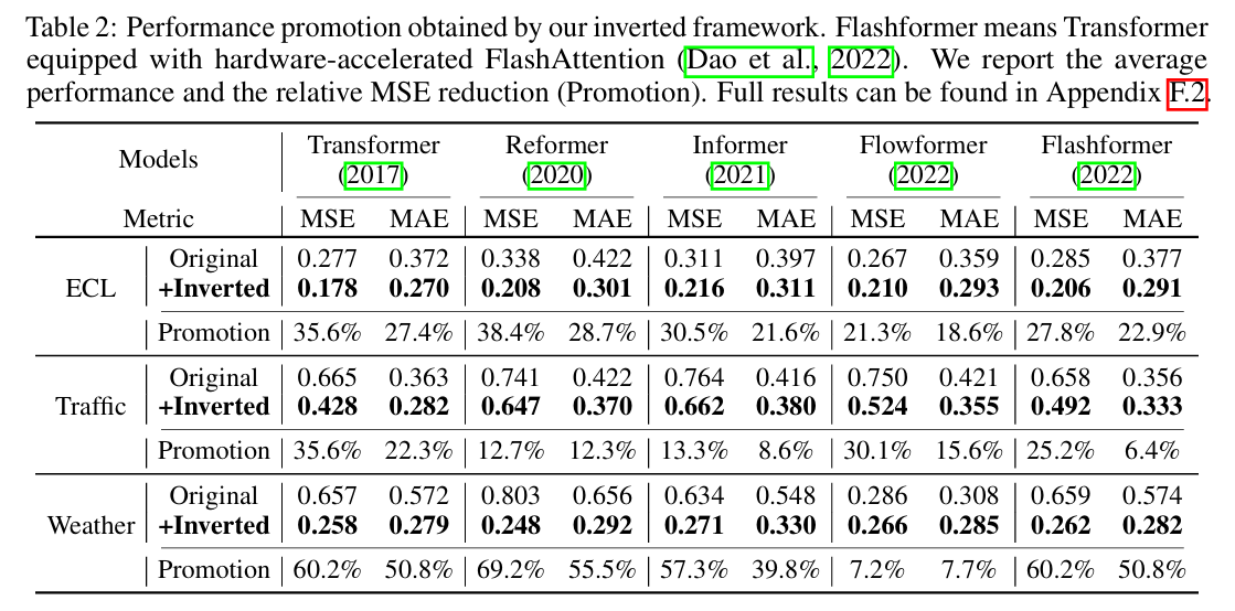
由于硬件为一台笔记本的3060显卡，写了一个测试脚本测试model里的各模型在weather、exchange、traffic三个数据集上的表现，测试了Flashformer、Folwformer、Informer、Reformer、Transformer五个模型以及对应的Inverted模型的效果。可以看出在使用inverted之后的预测mae和mse都出现了大幅度下降。测试的参数为epoch为1，其他的模型参数设计使用代码默认的网络大小。

问题：在使用traffic数据集进行测试的时候，会出现永远跑不出结果的问题，观察任务管理器发现，内存为100%，磁盘读取为100%。经过多次的观察和测试，减小–batch_size至4没有效果，因为问题出现在测试阶段。修改–num_workers至1或0也无效果。

目前想法：traffic数据集有862个特征，在写入结果的时候可能没有相应的优化。

消融实验

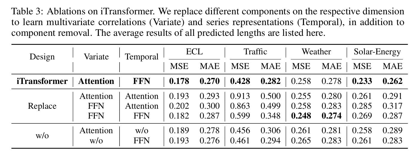
表3：iTransformer 的消融实验。我们在对应的维度上替换不同的组件，以学习多变量间的相关性（变量维，Variate）和序列表示（时间维，Temporal），同时也进行了组件移除的实验。此处列出了所有预测长度的平均结果。

消融实验是深度学习中验证模型各组件重要性的关键方法

在iTransformer的消融实验中，设计了以下几种变体：

1. 组件替换实验（Replace）：用不同的组件替换原始设计

2. 组件移除实验（w/o）：完全移除特定组件观察性能变化注意力机制（Attention）的作用

在iTransformer中，注意力机制被应用于变量维度而非时间维度。这种设计有以下关键作用：

捕获多变量相关性：注意力分数矩阵能够展现变量对之间的相关性，高度相关的变量会获得更高的权重

增强可解释性：生成的注意力图能够直观显示变量间的依赖关系，便于模型分析和理解

自适应加权：根据变量间的相似度动态调整信息交互的权重

FFN在iTransformer中承担时间序列表征学习的重要职责

时间模式提取：通过多层感知机提取复杂的时间序列表征，包括幅度、周期性和频谱特征

通用逼近能力：基于通用逼近定理，FFN能够学习描述任意时间序列的复杂表征

序列编码解码：在堆叠的反转块中，FFN负责编码观测序列并解码预测结果

为了测试的速度，该段仅选择weather作为实验数据集，选择{96，192}预测长度对这6种模型结构进行测试，epoch定为3。

weather测试结果：

experiment_name	description	pred_len	epochs	mse	mae
baseline	iTransformer (Variate: Attention, Temporal: FFN)	96	3	0.178201	0.218101
baseline	iTransformer (Variate: Attention, Temporal: FFN)	192	3	0.229345	0.262623
replace_variate_ffn	Variate: FFN, Temporal: Attention	96	3	0.186211	0.224299
replace_variate_ffn	Variate: FFN, Temporal: Attention	192	3	0.232352	0.261786
replace_temporal_attn	Variate: Attention, Temporal: Attention	96	3	0.180064	0.221066
replace_temporal_attn	Variate: Attention, Temporal: Attention	192	3	0.229681	0.262287
replace_both_ffn	Variate: FFN, Temporal: FFN	96	3	0.184406	0.222732
replace_both_ffn	Variate: FFN, Temporal: FFN	192	3	0.231027	0.260396
wo_variate_attn	Variate: w/o Attention, Temporal: FFN	96	3	0.186007	0.224726
wo_variate_attn	Variate: w/o Attention, Temporal: FFN	192	3	0.23217	0.263051
wo_temporal_ffn	Variate: Attention, Temporal: w/o FFN	96	3	0.182007	0.222693
wo_temporal_ffn	Variate: Attention, Temporal: w/o FFN	192	3	0.23222	0.264514

从测试结果来看，Baseline性能最佳，在 96 预测长度下，baseline 的 MSE 和 MAE 都是最低的，说明 Attention + FFN 组合在较短期预测中效果最好。

该数据集似乎不是非常明显地显示，所以增加数据集对比，接下来对solar数据集进行测试：

experiment_name	description	pred_len	epochs	mse	mae
baseline	Transformer (Variate: Attention, Temporal: FFN)	96	3	0.214071453	0.256544
baseline	iTransformer (Variate: Attention, Temporal: FFN)	192	3	0.251759768	0.283052
replace_variate_ffn	Variate: FFN, Temporal: Attention	96	3	0.253553808	0.291051
replace_variate_ffn	Variate: FFN, Temporal: Attention	192	3	0.284123659	0.30497
replace_temporal_attn	Variate: Attention, Temporal: Attention	96	3	0.234032243	0.282599
replace_temporal_attn	Variate: Attention, Temporal: Attention	192	3	0.273650736	0.306216
replace_both_ffn	Variate: FFN, Temporal: FFN	96	3	0.251736045	0.285938
replace_both_ffn	Variate: FFN, Temporal: FFN	192	3	0.282103747	0.301334
wo_variate_attn	Variate: w/o Attention, Temporal: FFN	96	3	0.238287553	0.278001
wo_variate_attn	Variate: w/o Attention, Temporal: FFN	192	3	0.279144794	0.298556
wo_temporal_ffn	Variate: Attention, Temporal: w/o FFN	96	3	0.238138705	0.287383
wo_temporal_ffn	Variate: Attention, Temporal: w/o FFN	192	3	0.276431978	0.307098

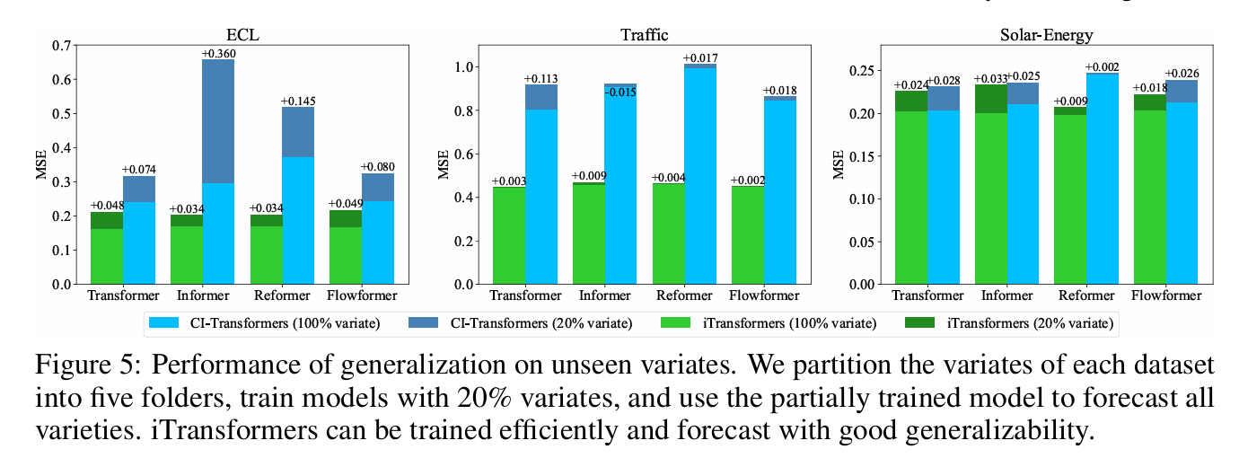
泛化性实验

20%样本测试：

实验名称	预测长度	MAE	MSE
ETTh1	96	0.4625	0.4440
ETTh1	192	0.5092	0.5212
ETTh2	96	0.3116	0.2086
ETTh2	192	0.3369	0.2424

100%样本测试：

实验名称	预测长度	MAE	MSE
ETTh1	96	0.4531	0.4396
ETTh1	192	0.4955	0.4999
ETTh2	96	0.2948	0.1920
ETTh2	192	0.3259	0.2273

测试说明：模型结构均使用默认参数，epoch为3。

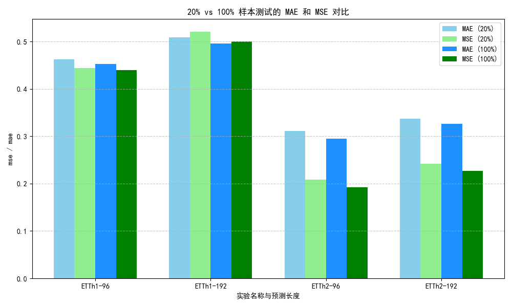
对比100%和20%的MAE和MSE数据，100%的训练样本仅仅有少量提高，说明iTransformer的泛化性能较好。

iTransformer部分预测结果可视化

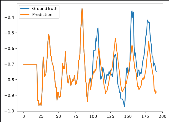
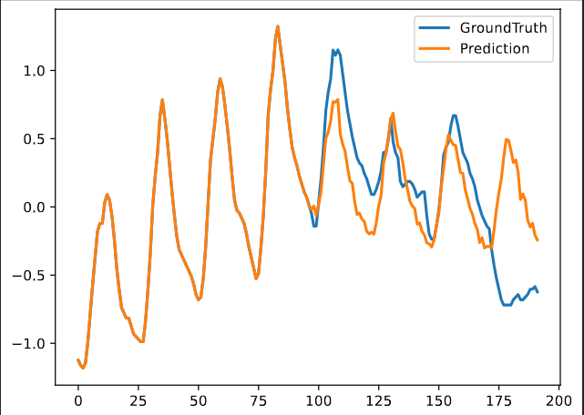
输入序列长度的影响

实验名称	MAE	MSE
ECL_48_96_iTransformer	0.27252841	0.18942103
ECL_96_96_iTransformer	0.24591123	0.15347210
ECL_192_96_iTransformer	0.23394144	0.13788573
ECL_336_96_iTransformer	0.23031704	0.13295323
ECL_720_96_iTransformer	0.23302031	0.13504007

学习

测试脚本设计

Repo里的.sh文件在windows环境下无法执行，转成.bat批处理文件来在windows环境下执行，具体如下

• 将 export CUDA_VISIBLE_DEVICES=0 更改为 set CUDA_VISIBLE_DEVICES=0。
• 将 model_name=iTransformer 更改为 set model_name=iTransformer。
• 将所有对 $model_name 的引用更改为 %model_name%

.npy文件

发现存储结果的文件夹特别大：

.npy是numpy数组形式的测试数据

        np.save(folder_path + 'metrics.npy', np.array([mae, mse, rmse, mape, mspe]))
        np.save(folder_path + 'pred.npy', preds)
        np.save(folder_path + 'true.npy', trues)

学习如何编写模型代码

class Model(nn.Module):

    def __init__(self, configs):

    def forecast(self, x_enc, x_mark_enc, x_dec, x_mark_dec):

    def forward(self, x_enc, x_mark_enc, x_dec, x_mark_dec, mask=None):

由于项目中有原始的Transformer实现，根据Attention is all you need论文中的实现，学习如何实现一个

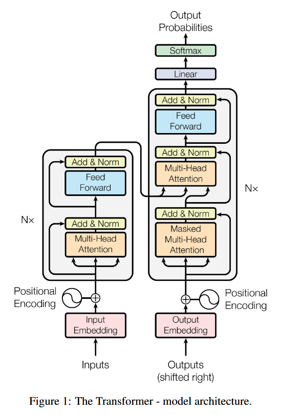
Input首先经过Embedding层：

# Embedding
        self.enc_embedding = DataEmbedding(self.enc_in, configs.d_model, configs.embed, configs.freq,
                                           configs.dropout)

然后经过encoder

# Encoder
        self.encoder = Encoder(
            [
                EncoderLayer(
                    AttentionLayer(
                        FullAttention(False, configs.factor, attention_dropout=configs.dropout,
                                      output_attention=configs.output_attention), configs.d_model, configs.n_heads),
                    configs.d_model,
                    configs.d_ff,
                    dropout=configs.dropout,
                    activation=configs.activation
                ) for l in range(configs.e_layers)
            ],
            norm_layer=torch.nn.LayerNorm(configs.d_model)
        )

具体有Attention层，FeedForward，Dropout与激活，LayerNorm。

然后是decoder

# Decoder
        self.dec_embedding = DataEmbedding(self.dec_in, configs.d_model, configs.embed, configs.freq,
                                           configs.dropout)
        self.decoder = Decoder(
            [
                DecoderLayer(
                    AttentionLayer(
                        FullAttention(True, configs.factor, attention_dropout=configs.dropout,
                                      output_attention=False),
                        configs.d_model, configs.n_heads),
                    AttentionLayer(
                        FullAttention(False, configs.factor, attention_dropout=configs.dropout,
                                      output_attention=False),
                        configs.d_model, configs.n_heads),
                    configs.d_model,
                    configs.d_ff,
                    dropout=configs.dropout,
                    activation=configs.activation,
                )
                for l in range(configs.d_layers)
            ],
            norm_layer=torch.nn.LayerNorm(configs.d_model),
            projection=nn.Linear(configs.d_model, configs.c_out, bias=True)
        )

内部按configs.d_layers叠加DecoderLayer，每层包含：Masked Attention、Cross Attention（Encoder-Decoder Attention）、FeedForward、Dropout与激活、LayerNorm。

对于Attention机制的疑问

问题1：为什么Attention机制可以用于时间序列预测？

问题2：许多人讲解Attention，每一个token（词）都有一个向量，那么模型要存储所有token 的向量吗？Attention迁移到时间序列预测上，对应的定义是什么？

问题3：为什么Transformer模型需要三个attention模块？

下一步规划

1.深入理解各个模块的作用、原理和实现。

2.从ITransformer的论文出发复现学习引用文献中的模型和实验。